Confidence Intervals

Mathematica Setup

This section is used to prepare Mathematica for this application, most notably by loading the Statistics and selected Graphics functions.

In[1]:=

Definition of Computational Formulæ

This section defines formulæ used in the actual computations, including the probability density functions for the Student T and distributions, and functions to return the critical values for those distributions.  In essence, these definitions import the relevant work that has been done in the Nine-Property notebooks for the distributions in a form convenient for this purpose.

Define Probability Density Functions

In[32]:=

Check the definitions by plotting the PDFs and inspecting the result to ensure that it is reasonable.

In[37]:=

Define Functions for Critical Values

Cadets are expected to find the critical values based on the percentile examples defined in the 9-property workbooks that are defined for each distribution.  In those workbooks, the percentile is defined in terms of finding a root of the cumulative distribution function, which is computationally expensive and can be somewhat finicky in Mathematica. A function definition for the critical value based on this principle might look somthing like this (for the T-distribution):

In[9]:=

Now perform a sample calculation whose result is known as a check.

In[10]:=

Out[10]=

Here, however, we elect to define the critical value functions in terms of the functions provided in the Statistics package, which are faster and less prone to numerical difficulties.

In[42]:=

Both approaches should give the same result.

In[13]:=

Out[13]=

Computing Confidence Intervals

Data Set Definition

This workbook can be used either as defined, with the sample values given directly, or by defining the sample statistics (in which case the definitions would be modified below).

In[14]:=

Out[14]=

The data displayed above are the heights of 11 male cadets.

Compute Relevant Sample Statistics

In[15]:=

Out[15]=

Out[16]=

Out[17]=

Define the Confidence Level

Define the confidence level as 100(1-α)% .

In[18]:=

Out[18]=

Confidence Interval on the Mean

Compute a 100(1-α)% confidence interval for the population mean, assuming the sample is from a population that is Normal with unknown standard deviation.

First using the standard formula defined in Devore.

In[20]:=

Out[20]=

and again using the Mathematica-defined functions in the Statistics package.

In[21]:=

Out[21]=

Crosscheck: the sample mean should be in the middle of this CI

In[22]:=

Out[22]=

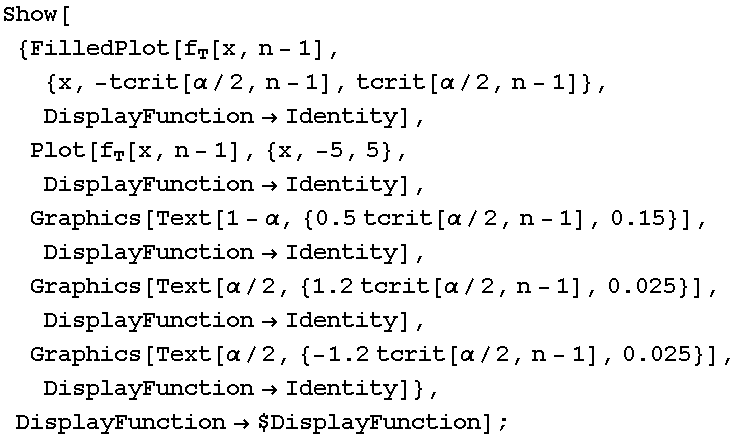
Now display a graph of the T-distribution with the area involved in the confidence interval shaded.

The Mathematica commands involved in this display are somewhat beyond those normally used by cadets

In[23]:=

Confidence Interval on the Variance and Standard Deviation

Compute a 100(1-α)% confidence interval for the variance, assuming the sample is from a population that is Normal.

In[24]:=

Out[24]=

and again using the Mathematica-defined functions in the Statistics package.

In[25]:=

Out[25]=

Both methods should, of course, give the same answer.

Confidence interval on the standard deviation is just the square root of the CI on the variance.

In[26]:=

Out[26]=

In[27]:=

Out[27]=

Crosscheck: the sample standard deviation should be in the middle of this CI

In[28]:=

Out[28]=

In[38]:=

A Simulation of Multiple Confidence Intervals to Assist in Understanding the Meaning of a Confidence Interval

Purpose

This simulation is intended to assist in understanding the concept of a confidence interval by providing the opportunity to do something that rarely happens in real life: computing many confidence intervals for the same parameter from different random samples of the same population.

A confidence interval is an "interval of plausible values" for a population parameter (Devore, p. 281).  By the nature of its definition, if many confidence intervals (based on different random samples from the same population) are computed, the fraction of those confidence intervals that cover the true population parameter should be about equal to the confidence level of the confidence intervals.  In other words, if we compute 1000 confidence intervals on the mean of a distribution with a confidence level of 90%, about 900 of them should cover the true population mean, and about 100 of them should miss the true value.

Summary

In this paper, we construct a simulation of  drawing a random sample from a normal (Gaussian) distribution and computing a confidence interval on the population mean from that sample.  As expected, for a 90% confidence level, about 90% of the resulting confidence intervals actually cover the true population mean.

Problem Setup

For the sake of specificity, consider the distribution of the height of a randomly selected cadet at the United States Military Academy. Based on both general considerations, and using this distribution as an example in several such classes, there is reason to believe that this population follows a normal distribution with mean about 70 inches and standard deviation about 5 inches.

In[1]:=

Since the usual class of cadets contains between 12 and 18 cadets, we will pretend that we are examining a sample consisting of a section of 15 cadets.

Finally, we will compute 90% confidence intervals on the mean, using "MeanCI".  However, for convenience in programming Mathematica, we will define our own function, "confidenceInterval" which takes exactly one arguement, the sample itself, and returns the confidence interval.  The trailing test ("ListQ") is designed to ensure that the function will fail if presented with an inappropriate arguement.

Simulation Construction

A Single Replication

For the sake of clarity, let's work through the manipulations needed for a single replication of the simulation.

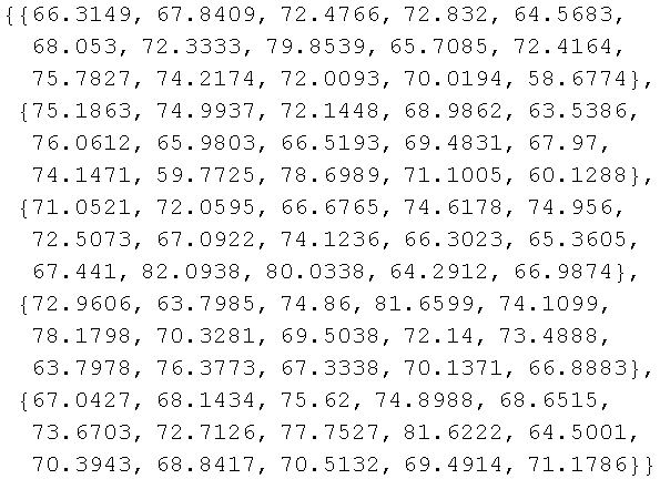
To begin with, we need to create the random sample from which we will compute the confidence interval.  We use the "RandomArray" function to create a matrix (with two rows) containing the appropriate sample

Since these are samples from a normal (Gaussian) distribution whose true mean and standard deviation are unknown (at least to the actual statistician), the appropriate form of the confidence interval is that based on the Student's T distribution.  As discussed above, we have embedded the Mathematica function in the user-defined function "confidenceInterval".

Now we have the confidence intervals, and we need to determine if the true mean is covered by those interval.

(Note: the approach to counting the successful intervals with "Select" is taken from Abell et al., page 356. The general form of this example was inspired by that section, although the specific details were created for this document.)

The number of "successful" confidence intervals is

while the total number of confidence intervals computed is

Therefore, the fraction of successful trials (confidence intervals that in fact cover the true mean) is

Inspection of the random data generated in the example indicates that this is a correct assessment, so we procede to a larger simulation.

Full Simulation Setup

For simplicity, we will set the number of replications to 1000:

Now we follow the same procedure as in the small scale example (the "Take" function is used to show a small set of the larger result):

Simulation Results

The fraction of the confidence intervals that in fact cover the true population mean, μ, is thus

Since we were computing confidence intervals with a confidence level of  

this is the standard to which the simulation results should be compared.  The fraction below shows the percentage error in the simulation --- the percentage the observed result differs from the expected result.

Each time this notebook is evaluated, the results will change.  However, the values computed in the intial versions of this notebook were 0.888 and 0.899. Both of these are reasonably close to the (then) expected value of 0.90  (-1.2% and -0.1%, respectively).

Conclusions

This simulation demonstrates that the theoretically expected result of taking many samples from the same population and computing the confidence interval from each is achieved.  When this procedure is followed, about the fraction of the confidence intervals predicted by the confidence level do in fact cover the true population parameter (in this case the population mean).

Construction of this simulation in Mathematica is somewhat beyond the capabilities expected of students in the basic Probability and Statistics course. In particular, the use of the "Map" and "Select" functions to iterate over the array of samples, and the use of the "MeanCI" function to compute the confidence interval in one step are beyond the Mathematica programming taught in the course.  

However, the basic concepts embodied in this simulation should be reasonably clear.  If we take many random samples from the same population and compute confidence intervals for the population parameter from them, some will cover the true mean, and some will not.  The fraction of the confidence intervals that do cover the true mean is random, but in the long run will be about the percentage defined by the confidence level used in the creation of the confidence intervals.  That is what we mean when we say "I am 90% confidence that the true average height of cadets is between  67.6778 and 71.7354 inches."

Created by Mathematica  (July 20, 2006)