Empirical Distribution Functions

Mathematica Overview

This section discusses the mechanics of plotting and manipulating Empirical Distribution Functions (EDF) in Mathematica.

Since this subject is best discussed with the aid of an example, we start by creating the array of data for which we want to plot the EDF. This example is taken from Project II as presented during STAP 04. I have significantly reduced the number of replications in order to be able to show the data without taking too much space.

In[13]:=

In[15]:=

Out[15]=

Note: this section uses a number of the more advanced Mathematica manipulations available with the Statistics and DataManipulation packages; the principles involved are straightforward, but the manipulations may not be.

Now what we need to do is to create a matrix with the sorted values of the sample each appearing twice in the first column, and the frequency data appearing in the second column.  The exact organization of the data is intended to cause the plotting routines to plot it as a step function.

First, create a vector (list) of the frequency values.  This list consists of the values {0, 1/n, 1/n, 2/n, 2/n, 3/n, 3/n, ... , (n-1)/n, (n-1)/n, 1}.  We create it by first creating a list of the values {1/n, 2/n, ..., 1}

In[16]:=

Out[16]=

Then we double the list and insert the value 0, converting the nested lists into a single flat list

In[17]:=

Out[17]=

Notice that every value appears twice except 0.  Now we sort the list and remove one of the 1's at the top of the list, assigning the result to a symbol "freq".

In[36]:=

Out[36]=

Each value in the sample also appears twice, and needs to be sorted;

In[19]:=

Out[19]=

If we simply make a list of the two lists, we will have a matrix with the right values in it.  However, the list will consist of two rows and n columns, while we want it to be two columns and n rows.  The Transpose function takes care of this.

In[20]:=

Out[20]=

Now we can plot the resulting pairs.  The "PlotJoined→True" option causes Mathematica to join the plotted points with line segments, which is the desired form of the plot.

In[21]:=

Out[21]=

Fitting A Model to the EDF

Once the EDF has been constructed, we need to fit a model of some sort to it.  The fundamental process is to select parameters for the model that cause it to fit "well" to the data; there are several ways to approach this problem.

Estimator Approach

One approach to this problem is one that fits (pun intended) well with traditional statistics: define an estimator for the parameter(s) in question and use the point estimates resulting from it.  In this case, we will try to fit the Gamma distribution, finding point estimates for E(X) = αβ and V(X) =

In[22]:=

Out[22]=

In[23]:=

Out[23]=

In[24]:=

Out[24]=

These are our estimates for α and β; check to make sure they really have the desired properties (which is mostly a check that we did the solution right).

In[25]:=

Out[25]=

In[26]:=

Out[26]=

Plot the fitted graph

In[27]:=

And now the fit and the EDF on the same axis.

In[28]:=

Out[28]=

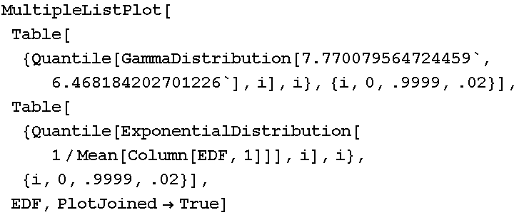
Clearly this is a reasonably good fit of the distribution; since it's part of Project II, let's apply the same technique to an exponential.

In[29]:=

Out[29]=

Clearly, while it may have the same mean, the exponential distribution is not as good a model of the simulated data as the Gamma distribution.

Least Squares Fit

In principle, computation of the least squares fit is straightforward; the actual Mathematica implementation is much less straightforward..

The first step is to find the predicted values corresponding to the observed values.

In[35]:=

Out[35]=

In[73]:=

Out[73]=

Compare the predictions and observed values

In[78]:=

Out[78]=

Compute the sum of squared errors.  

In[86]:=

Out[86]=

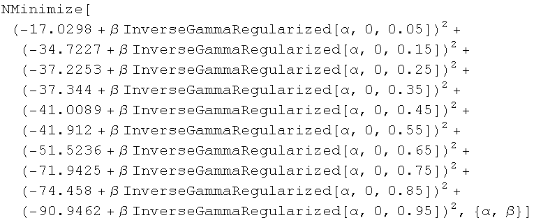
Finally, minimize the sum of the squared error as a function of the family parameters.

In[85]:=

Out[85]=

In[84]:=

In[228]:=

Out[228]=

In[229]:=

Out[229]=

In[230]:=

Out[230]=

In[231]:=

Out[231]=

Created by Mathematica  (July 20, 2006)